 |
| Figure 1. Left: Time- and longitudinally averaged wind-stress. Right: Contours of oceanic mass transport (in black) and contours of sea surface temperatures (in colors). The transport of sea surface temperatures by the oceanic currents creates a thermal front beneath the westerlies' maximum. |
The large-scale oceanic currents that redistribute heat, salt and momentum in the top kilometer of water are driven by the mechanical stress exerted by the winds at the air-sea interface. In turn, the surface winds are shaped by the north-south temperature differences in the atmosphere. The temperature gradients in the atmosphere, largely determined by the sun's differential heating, are mitigated by the poleward heat transport due to the oceanic currents and the atmospheric flows. Thus, the ocean and the atmosphere work together to make our planet livable.
Understanding the partitioning of heat transport between atmospheric and oceanic components, and how fluctuations arise because of the mutual interaction of the two systems, is a crucial aspect of climate dynamics. One approach is to construct simple models based on fundamental conservation principles of heat, salt and momentum. An example of oceanic and atmospheric fields resulting from one such model is shown in figure 1.
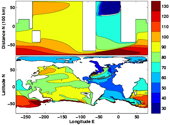 |
| Figure 2. The time of arrival of the first maximum in SSH in response to a change in the northern North Atlantic is contoured in years. White areas are either continents or values outside the contoured range. (Top) A solution of a one-layer model of the World Ocean in simplified geometry, forced in the northernmost North Atlantic by a thickness anomaly with a period of 100 years. (Bottom) Corresponding results for the SSH anomalies in a three-dimensional OGCM forced by wind and buoyancy gradients. The SSH anomalies are the difference between a perturbed experiment (where deep convection is interrupted in the Labrador Sea by a local anomalous freshwater flux) and a control experiment (similar to modern observation). The anomalous freshwater flux is a sinusoid in time with a period of 100 years. |
The global adjustment of the upper ocean in response to localized anomalies is effected by planetary waves which propagate from one basin to another in several decades. Planetary ocean waves give rise to a global seiche, such that the volume of thermocline water decreases in the Pacific-Indian Ocean while increasing in the Atlantic Ocean.
The propagation of a disturbance from the North Atlantic is illustrated in figure 2, where the arrival times of the first maximum of sea-surface height (SSH) are shown. From the source region in the North Atlantic a wave propagates equatorward along the American coast. At the equator it moves eastward and then splits into two waves moving north and south along the eastern boundary of the Atlantic. At the southern tip of Africa the wave turns eastward until it finds its way to the Indian and the Pacific oceans. The wave acts like the El Nińo, travelling eastward along the equator until it penetrates poleward along the eastern boundary. From there, the disturbance is radiated westward in the form of slower Rossby waves that 60 years after the initial North Atlantic anomaly fill the entire basin.
A salt flux perturbation in the North Atlantic generates a global
seiche which may trigger an El Nińo in the equatorial Pacific several
decades later.
Reprints of recent articles:
- P. Cessi, F. Primeau: Dissipative selection of low-frequency modes in a reduced-gravity basin. (PDF file: 727Kb)
- P. Cessi: Thermal feedback on wind-stress as a contributing cause of climate variability.
(PDF file: 336Kb)
- B. Gallego, P. Cessi: Exchange of heat and momentum between the atmosphere and the ocean: a minimal model of decadal oscillations.
(PDF file: 410Kb)
- F. Primeau and P. Cessi: Coupling between wind-driven currents and midlatitude storm tracks. (PDF file: 390Kb)
- P. Cessi and S. Louazel: Decadal oceanic response to stochastic wind forcing. (PDF file: 301Kb)
- B. Gallego and P. Cessi: Decadal Variability of Two Oceans and an Atmosphere.
(PDF file: 635Kb)
- P. Cessi and F. Paparella: Excitation of basin modes by ocean-atmosphere
coupling. (PDF file: 190Kb)
- R. Ferrari and P. Cessi: Seasonal synchronization in a chaotic
ocean--atmosphere model. (PDF file: 300Kb)
- M. Spydell and P. Cessi: Baroclinic modes in a two-layer basin.
(PDF file: 2Mb)
- P. Cessi and P. Otheguy: Oceanic teleconnections: remote response to decadal wind forcing. (PDF file: 1.1Mb)
- P. Cessi, K. Bryan and R. Zhang: Global seiching of
thermocline waters between the Atlantic and the Indian-Pacific Ocean
basins. (PDF file: 230Kb)
- B. Gallego, P. Cessi and J.C.McWilliams: The Antarctic
Circumpolar Current in equilibrium. (PDF file: 439Kb)
- P. Cessi and M. Fantini: The eddy-driven thermocline. (PDF file: 301Kb)
- P. Cessi, W.R. Young and J.A. Polton: Control of large-scale heat transport by small-scale
mixing. (PDF file: 880Kb)
- P. Cessi: Regimes of thermocline scaling: the
interaction of wind-stress and surface buoyancy. (PDF file: 500Kb)
- P. Cessi: An energy-constrained parametrization of eddy buoyancy flux. (PDF file: 500Kb)
- Wolfe, C. L., P. Cessi, J. L. McClean, and M. E. Maltrud: Vertical heat transport in eddying ocean models. (PDF file: 174Kb)
- Wolfe, C. L. and P. Cessi: Overturning Circulation in an Eddy-Resolving Model: The Effect of the Pole-to-Pole Temperature Gradient. (PDF file: 2.57Mb)
- P. Cessi and Wolfe, C. L.: Eddy-driven buoyancy gradients on eastern boundaries and their role in the thermocline (PDF file: 1.3Mb)
- P. Cessi, Wolfe, C. L. and Ludka, B.C.: Eastern-boundary contribution to the Residual and Meridional Overturning Circulations\
aries and their role in the thermocline (PDF file: 1.3Mb)
- Wolfe, C. L. and P. Cessi: What Sets the Strength of the Mid-Depth Stratification and Overturning Circulation in Eddying Ocean Models? (PDF file: 2.57Mb)
- Wolfe, C. L. and P. Cessi: The adiabatic pole-to-pole overturning circulation (PDF file: 2.Mb)
- Cessi P. and C. L. Wolfe : Adiabatic eastern boundary currents (PDF file: 3.4Mb)
- Cessi, P. and N. Pinardi and V. Lyubarstev : Energetics of Semienclosed Basins with Two-Layer Flows at the Strait (PDF file: 0.9Mb)
- Wolfe, C.L. and P. Cessi: Salt Feedback in the Adiabatic Overturning Circulation (PDF file: 2.9Mb)
- Abernathey, R. and P. Cessi P.: Topographic Enhancement of Eddy Efficiency in Baroclinic Equilibration (PDF file: 3.6Mb)
- Wolfe, C.L. and P. Cessi: Multiple Regimes and Low-Frequency Variability in the Quasi-Adiabatic Overturning Circulation (PDF file: 6.7Mb)
- Jones, C.S. and P. Cessi: Interbasin transport of the meridional overturning circulation (PDF file: 3.3Mb)
Publication list